COMP562-2022-Group-1.github.io

A Machine Learning Project for UnC COMP562

COMP 562 Project

Relevant Links

Introduction

In this paper, we will take a closer look at a 2016 post-elections survey conducted by the Latin American Public Opinion Project. The purpose of this paper is to identify which factors are more important in deciding which candidate a voter votes for. This can be useful in helping the candidates and their parties decide on their target audience in order to help them carry out their future campaigns efficiently, and also their future policy stand to attract more voters to vote for them.

The questionnaire is available here, with questions on trust in government, opinions on public policies and political lean.

The source code for the preprocessing the data and training the model is available on Github.

The survey is conducted by the Latin American Public Opinion Project (LAPOP) 1. The AmericasBarometer is the only scientifically rigorous survey of democratic public opinion and behavior that covers the Americas. The results of AmericasBarometer and other surveys conducted by LAPOP are used by researchers and government practitioners to investigate democracy and develop public policies. An example is the strong evidence from the 2004 AmericasBarometer survey that Honduras has been politically unstable, long before the 2009 crisis.

Data Preprocessing

The United States Online Survey data for 2017 is stored in a csv file that is accessible from the LAPOP website. The data contains 70 variables, which are answers to questions in the questionnaire. All of these are categorical variables. With too many na' responses to question numbers q12m’ and q12f' and sinceq1’ and q2' were not present in the questionnaire, they were removed. v3bn’ was also extracted and removed as it contained the output of which president was voted for. This left us with 65 variables.

Removing Redundant Variables

Next, the colinearity between the variables was analyzed. For variable pairs with high absolute colinearity of at least 0.9, one variable can be dropped. There was one such variable pair, so one variable was dropped, leaving 64 variables.

Encoding Categorical Values

The inputs are encoded as dummy variables for questions with multiple answers that could not be measured on a scale. For example, q11n: What is your marital status? has 7 possible values and was represented by 6 dummy variables.

Stratified Sampling

Stratified sampling is used to perform the train-test split so that the training and test datasets contain the same ratio of classes. A 80-20 split was done to determine the train-test sets.

Oversampling

The training set has a significantly greater proportion of units with labels 2 and 3 compared to the other labels. Synthetic Minority Oversampling Technique (SMOTE) is used to balance out the minority labels in the training set by creating synthetic observations through considering the k-nearest neighbours in the feature space of the present observations. This is done in order to ensure that the models are not distorted during training due to the imbalance class labels.

Modelling

eXtreme Gradient Boosting Classifier Model

This ensemble model uses a gradient descent algorithm to minimize the loss function when adding new models to the ensemble. Maximum tree depth of 5 is used to prevent over-fitting. The number of boosting rounds is set to 240 and the learning objective is set to multiclass softprob.

Random Forest Classifier Model

This model is an ensemble of 200 decision trees of maximum depth 6. The maximum depth prevents the decision trees from over-fitting. The quality of split at each node of a decision tree is determined using entropy.

Logistic Regression Model

A logistic function is evaluated on a linear combination of features to compute the probability of a class. The saga solver is used to minimize the multinomial loss within a maximum of 2000 iterations.

Ensemble Model

Uses an ensemble of the XGBoost, Random Forest and Logisitic Regression classifiers. The class label is predicted by summing the predicted probabilities of each label over all models and returning the label with the largest sum.

Model Evaluation

The models are evaluated using precision, recall (true positive rate), accuracy, f1 score and Area Under the Receiver Operating Characteristic Curve (AUC).

Precision

Precision is the proportion of correctly predicted positive cases to the total number of cases that were predicted as positive. $\textrm{Precision} = \frac{\textrm{TP}}{\textrm{TP} + \textrm{FP}}$

Recall

Recall is the proportion of the positive cases that were correctly predicted. $\textrm{Recall} = \frac{\textrm{TP}}{\textrm{TP} + \textrm{FN}}$

Accuracy

Accuracy is the proportion cases that were correctly predicted. $\textrm{Accuracy} = \frac{\textrm{TP} + \textrm{TN}}{\textrm{TP} + \textrm{FN} + \textrm{FP} + \textrm{TN}}$

F1 Score

F1 score is the harmonic mean of the precision and recall. $\textrm{F1 Score} = 2 \times \frac{\textrm{Precision} \times \textrm{Recall}}{\textrm{Precision} + \textrm{Recall}}$

AUC

The Receiver Operating Characteristic (ROC) curve plots recall against false positive rate for each classification threshold that changes the number of cases predicted as positive.

$\textrm{FPR} = \frac{\textrm{FP}}{\textrm{FP} + \textrm{TN}}$

A better model would have a larger value of $|\textrm{AUC} - 0.5|$ which indicates that the model would have a higher recall at any given false positive rate.

Discussion of Results

Table 1 (Results from evaluating the classification models)

Model	AUC	F1 Score	Accuracy	Precision	Recall
XGBoost	0.81453	0.81088	0.81696	0.81349	0.81969
Random Forest	0.83605	0.83834	0.83482	0.84874	0.83482
Logistic Regression	0.7623	0.79298	0.79018	0.79819	0.79018
Ensemble Model	0.81764	0.81972	0.82143	0.82292	0.82143

Table 1, the Random Forest model had the highest score for all five metrics used in evaluation. Therefore, the Random Forest model would be the most useful model among the five models for predicting the candidate a person would vote for given the person’s response to the United States Online Survey.

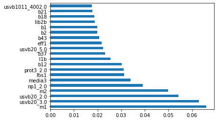
In addition to making predictions of the candidate that a voter is most likely to vote for, the models can also be used to identify the most important features that affect the candidate that a person votes for. For example, Figure 1a plots the top 20 most important features used in the Random Forest Classifier. Among the features plotted in the graphs below, the top 3 features are:

m1: Speaking in general of the current administration, how would you rate the performance of Donald Trump?
usvb20: If the next presidential elections were being held this week, what would you do?
m2: Now speaking of Congress, and thinking of members of Congress as a whole, without considering the political parties to which they belong, How well do you believe that the members of Congress are performing their jobs?


Figure 1a: Top 20 most important features used in the Random Forest Classifier


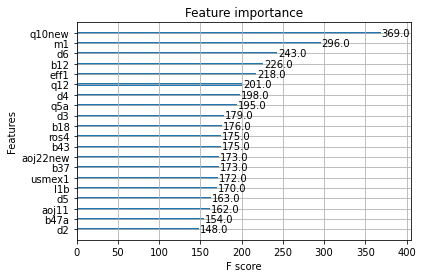Figure 1b: Features with the 20 highest coefficients in the XGBoost Classifier


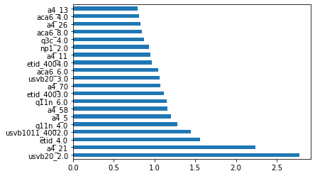Figure 2a: Features with the 20 highest coefficients for Hilary


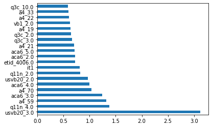Figure 2b: Features with the 20 highest coefficients for Trump

As previously mentioned, these models can be used by the candidates and parties to strategize their election campaigns and optimize their limited resources. Even though the logistic regression performed poorer in all of the performance metrics, it can still be used by each party to observe what demographics their opponents are attracting, and try to garner more swing votes by campaigning for the wants of the people.

References

The AmericasBarometer by the LAPOP Lab
Vanderbilt LAPOP Lab releases 2021 AmericasBarometer survey results
Mitchell A. Seligson, John A. Booth: Predicting Coups? Democratic Vulnerabilities, The AmericasBarometer and The 2009 Honduran Crisiss